- Introduction
- Set Up Your Environment
- Set up Working Environment
- The Analysis
- Read Filtering
- Learn the Error Rates and Infer Sequences
- Merge Forward and Reverse Reads
- Construct Sequence Table
- Remove chimeras
- Tracking Reads throughout Pipeline
- Assign Taxonomy Information
- Phyloseq Object
- Taxonomic Filtering
- Prevalence Filtering
- Visualization / Diversity
Introduction
The purpose of this post will be to guide researchers through a basic analysis of microbiome data using R packages DADA2 and Phyloseq. Most concepts will be discussed at a very high level and I won’t spend too much time digging into the weeds of the analysis. For more in-depth analysis, check out this pipeline tutorial which was heavily referenced when creating this tutorial.
We will be analyzing a very small subset of data that was used in part to look at differences in microbiome structure between mice given a regular diet (RD, n = 24) versus a diet with no isoflavones (NIF, n = 24). Fecal samples from each mouse were collected 2 weeks after being fed either the RD or NIF diets. Samples were processed in the lab and subjected to Illumina MiSeq 300 base paired-end sequencing. We specifically targeted the V4 variable region of the 16S rRNA gene for sequencing. Reads from each sample were subsampled to 5000 reads/sample just to make the data a bit more manageable.
Set Up Your Environment
Before we can get started, there are a few things you’ll need to download/install:
The Microbiome Data
The data has been compressed into a single tar.gz file. You’ll need to download it and de-compress it. This can usually be done by simply double-clicking on it.
Download the data here
You’ll also need the SILVA reference database in order to assign taxonomy information to each sequence. That is also contained within the above linke (silva_nr_v132_train_set.fa.gz).
Download and Install necessary R packages
In order to get DADA2, Phyloseq, and a few other packages installed on your computer, you need to install them from the internet. Some of these packages can take a while to install, so don’t be alarmed if it take a couple minutes. DADA2 and Phyloseq are held within Bioconductor, which a collection of packages used primarily for biological data analysis, so you’ll need to install Bioconductor prior to installing DADA2 and Phyloseq. Once all packags are installed, you won’t have access to them until you “turn them on” using the library() command.
DADA2: Please follow the directions from this website. This is the package that does much of the “heavy” lifting in terms of read quality processing and error rate detection.
Phyloseq: Please follow the directions from this website. This package is primarily used to process the high-quality reads, generate diversity statistics, and make pretty figures.
Tidyverse: This is a suite of packages that are used for variety of data science needs (read/write files, clean/edit data, make cool figures, etc). To install, simply enter
install.packages("tidyverse")into your R prompt.
These two blocks of code should install and load all of the packages needed:
# DADA2 install
if (!requireNamespace("BiocManager", quietly = TRUE))
    install.packages("BiocManager")
BiocManager::install("dada2", version = "3.10")

# Phyloseq install
if (!requireNamespace("BiocManager", quietly = TRUE))
    install.packages("BiocManager")
BiocManager::install("phyloseq")

# Tidyverse install
install.packages("tidyverse")

# KableExtra for pretty tables
install.packages("kableExtra")
# Load packages
library(dada2)
library(phyloseq)
library(tidyverse)
library(kableExtra)Set up Working Environment
Reads
To make things easier, we need to create some variables that will hold the names of our fastq files and the directory for our soon-to-be processed reads. The following code block will store the paths for the forward (R1) and reverse (R2) fastq files (raw and processed):
# Get path of directory that contains all of the reads
#  change if reads in separate file on your computer
reads_path <- "data/mouse_samples"

# Store path of forward and reverse reads
Fs_path <- sort(list.files(reads_path, pattern="R1.fastq", full.names = TRUE))
Rs_path <- sort(list.files(reads_path, pattern="R2.fastq", full.names = TRUE))

# Create directories for processed forward and reverse reads
Fs_path_filtered <- file.path(reads_path, "filtered_Fs")
Rs_path_filtered <- file.path(reads_path, "filtered_Rs")
Extract the sample names as well:
mouse_sample_names <- str_replace(string = basename(Fs_path),
                                  pattern = "_R1\\.fastq",
                                  replacement = "")
The Analysis
Check Read Quality
We first want to get a general idea of the quality of the reads in our dataset. Let’s look at a random subsampling of the samples:
set.seed(1234) # Ensures the same "random" sampling is performed

# Forward Read quality
plotQualityProfile(Fs_path[sample(1:48, 12, replace = FALSE)])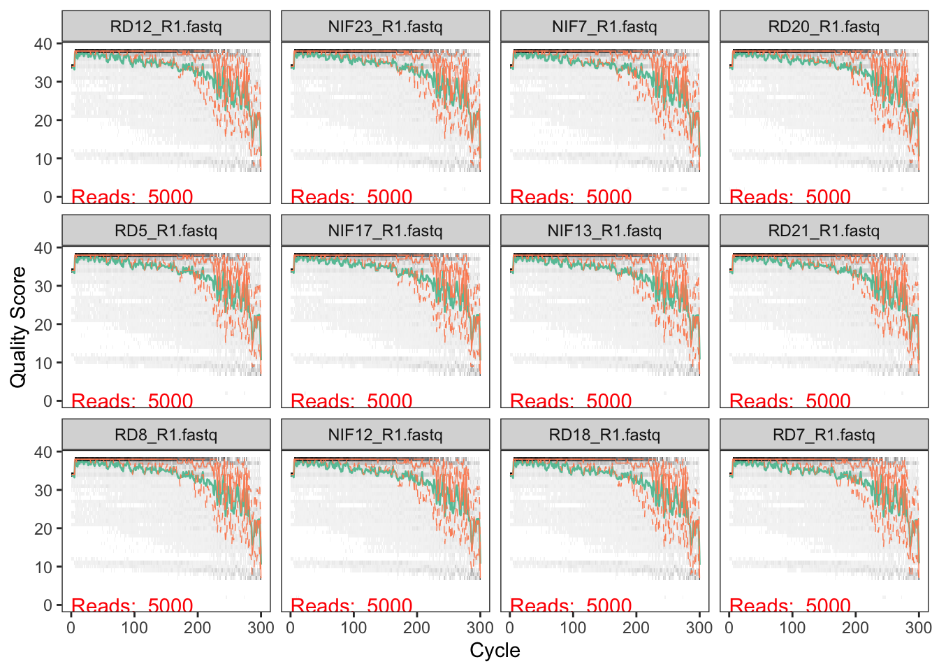
# Reverse Read quality
plotQualityProfile(Rs_path[sample(1:48, 12, replace = FALSE)])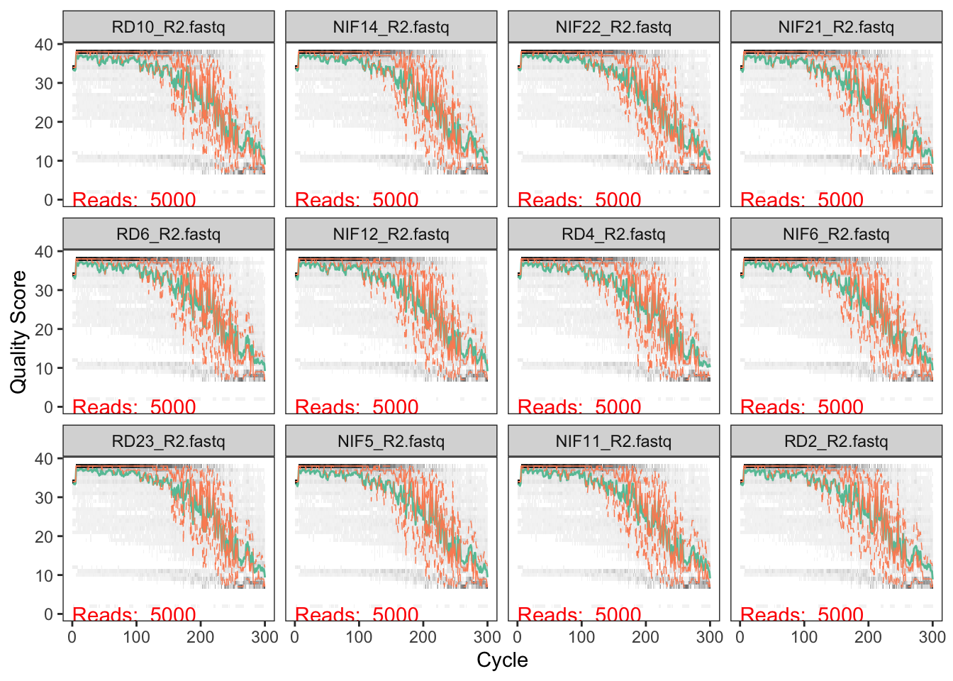
We typically don’t want to have the read quality drop below ~30 (focus on the green lines which represent mean quality). But we also need to make sure that our reads have sufficient overlap. The V4 region of the 16S rRNA gene is about 250bp in length, so if we decide to trim off the ends of the sequences due to low quality, the remaining lengths must be >250…actually it needs to be more than that in order to have sufficient overlap. I believe that DADA2 requires at least 12bp overlap, but the more the better.
For the forward reads, we see the quality drop at around 200bp. For the reverse reads, which are lower in quality (not atypical), we see the quality drop at around 150bp. We will use 200 and 150 to trim our seqeunces.
Read Filtering
Using the following parameters:
maxN=0(DADA2 requires no Ns)truncQ=2Truncate reads at the first instance of a quality score less than or equal to truncQ (keeping this as default)rm.phix=TRUE: discard reads that match against the phiX genomemaxEE=c(2,2): sets the maximum number of “expected errors” allowed in a read, which is a better filter than simply averaging quality scores.
out <- filterAndTrim(fwd=Fs_path,
              filt=Fs_path_filtered,
              rev=Rs_path,
              filt.rev=Rs_path_filtered,
              truncLen=c(200,150), # forward and reverse read
              maxEE=c(2,2),
              truncQ=2,
              maxN=0,
              rm.phix=TRUE,
              compress=TRUE,
              verbose=TRUE,
              multithread=TRUE)
out
## reads.in reads.out
## NIF1_R1.fastq 5000 4013
## NIF10_R1.fastq 5000 4137
## NIF11_R1.fastq 5000 4320
## NIF12_R1.fastq 5000 4075
## NIF13_R1.fastq 5000 4111
## NIF14_R1.fastq 5000 4370
## NIF15_R1.fastq 5000 4075
## NIF16_R1.fastq 5000 4317
## NIF17_R1.fastq 5000 4169
## NIF18_R1.fastq 5000 4108
## NIF19_R1.fastq 5000 4091
## NIF2_R1.fastq 5000 4121
## NIF20_R1.fastq 5000 4121
## NIF21_R1.fastq 5000 4061
## NIF22_R1.fastq 5000 4542
## NIF23_R1.fastq 5000 4203
## NIF24_R1.fastq 5000 4219
## NIF3_R1.fastq 5000 4358
## NIF4_R1.fastq 5000 4247
## NIF5_R1.fastq 5000 4260
## NIF6_R1.fastq 5000 4314
## NIF7_R1.fastq 5000 4066
## NIF8_R1.fastq 5000 4056
## NIF9_R1.fastq 5000 4071
## RD1_R1.fastq 5000 4173
## RD10_R1.fastq 5000 4264
## RD11_R1.fastq 5000 4276
## RD12_R1.fastq 5000 4208
## RD13_R1.fastq 5000 4272
## RD14_R1.fastq 5000 4189
## RD15_R1.fastq 5000 4390
## RD16_R1.fastq 5000 4182
## RD17_R1.fastq 5000 4529
## RD18_R1.fastq 5000 4135
## RD19_R1.fastq 5000 4090
## RD2_R1.fastq 5000 4103
## RD20_R1.fastq 5000 4253
## RD21_R1.fastq 5000 4214
## RD22_R1.fastq 5000 4357
## RD23_R1.fastq 5000 4539
## RD24_R1.fastq 5000 4212
## RD3_R1.fastq 5000 4230
## RD4_R1.fastq 5000 4341
## RD5_R1.fastq 5000 4233
## RD6_R1.fastq 5000 4231
## RD7_R1.fastq 5000 4121
## RD8_R1.fastq 5000 4244
## RD9_R1.fastq 5000 4272We can see from the output that for most samples, about 600-900 reads were removed from each sample. This seems pretty reasonable. If you find that most of your reads are being thrown out, then you may need to tweak your filtering parameters.
Let’s also rename the samples (so they don’t have the *_R1.fastq* ending):
# Get list of filtered sequences
Fs_filt <- list.files(Fs_path_filtered, full.names = TRUE, pattern = "fastq")
Rs_filt <- list.files(Rs_path_filtered, full.names = TRUE, pattern = "fastq")

# Create names
names(Fs_filt) <- mouse_sample_names
names(Rs_filt) <- mouse_sample_names
Learn the Error Rates and Infer Sequences
High throughput sequencing is not perfect…in fact is pretty error prone. Sometimes you’ll see workflows estimate their error rates by sequencing a mock community (which is a good idea). However, DADA2 leverages some statistical magic (a parametric error model) to estimate sequencing errors by comparing amplicons to the most abundant amplicons present in your sample. The default is to use 1x10⁸ (recommended), but to spead things up, I’ll use 1e7 reads.
# Forward read estimates
errF <- learnErrors(Fs_filt, nbases = 1e7, multithread=TRUE)
## 10805600 total bases in 54028 reads from 13 samples will be used for learning the error rates.# Reverse read estimates
errF <- learnErrors(Rs_filt, nbases = 1e7, multithread=TRUE)## 10025100 total bases in 66834 reads from 16 samples will be used for learning the error rates.Now that you’ve estimated the error rates, we need to go back to our samples and analyze each read and infer it’s true sequence given the error rates. Basically, it’s going to determine the number of unique reads per sample.
# Infer forward reads
dadaFs <- dada(Fs_filt, err=errF, multithread=TRUE)
## Sample 1 - 4013 reads in 1776 unique sequences.
## Sample 2 - 4137 reads in 1641 unique sequences.
## Sample 3 - 4320 reads in 1653 unique sequences.
## Sample 4 - 4075 reads in 1717 unique sequences.
## Sample 5 - 4111 reads in 1770 unique sequences.
## Sample 6 - 4370 reads in 1761 unique sequences.
## Sample 7 - 4075 reads in 1574 unique sequences.
## Sample 8 - 4317 reads in 1929 unique sequences.
## Sample 9 - 4169 reads in 1876 unique sequences.
## Sample 10 - 4108 reads in 1922 unique sequences.
## Sample 11 - 4091 reads in 1811 unique sequences.
## Sample 12 - 4121 reads in 1744 unique sequences.
## Sample 13 - 4121 reads in 1893 unique sequences.
## Sample 14 - 4061 reads in 1823 unique sequences.
## Sample 15 - 4542 reads in 1915 unique sequences.
## Sample 16 - 4203 reads in 1773 unique sequences.
## Sample 17 - 4219 reads in 1835 unique sequences.
## Sample 18 - 4358 reads in 1580 unique sequences.
## Sample 19 - 4247 reads in 1693 unique sequences.
## Sample 20 - 4260 reads in 1795 unique sequences.
## Sample 21 - 4314 reads in 1735 unique sequences.
## Sample 22 - 4066 reads in 1598 unique sequences.
## Sample 23 - 4056 reads in 1667 unique sequences.
## Sample 24 - 4071 reads in 1624 unique sequences.
## Sample 25 - 4173 reads in 1854 unique sequences.
## Sample 26 - 4264 reads in 1794 unique sequences.
## Sample 27 - 4276 reads in 2022 unique sequences.
## Sample 28 - 4208 reads in 1871 unique sequences.
## Sample 29 - 4272 reads in 1911 unique sequences.
## Sample 30 - 4189 reads in 1834 unique sequences.
## Sample 31 - 4390 reads in 1768 unique sequences.
## Sample 32 - 4182 reads in 1851 unique sequences.
## Sample 33 - 4529 reads in 1839 unique sequences.
## Sample 34 - 4135 reads in 1782 unique sequences.
## Sample 35 - 4090 reads in 1773 unique sequences.
## Sample 36 - 4103 reads in 1937 unique sequences.
## Sample 37 - 4253 reads in 1758 unique sequences.
## Sample 38 - 4214 reads in 1781 unique sequences.
## Sample 39 - 4357 reads in 2018 unique sequences.
## Sample 40 - 4539 reads in 1643 unique sequences.
## Sample 41 - 4212 reads in 1679 unique sequences.
## Sample 42 - 4230 reads in 2000 unique sequences.
## Sample 43 - 4341 reads in 1931 unique sequences.
## Sample 44 - 4233 reads in 1798 unique sequences.
## Sample 45 - 4231 reads in 1769 unique sequences.
## Sample 46 - 4121 reads in 1796 unique sequences.
## Sample 47 - 4244 reads in 1887 unique sequences.
## Sample 48 - 4272 reads in 1702 unique sequences.# Infer reverse reads
dadaRs <- dada(Rs_filt, err=errF, multithread=TRUE)## Sample 1 - 4013 reads in 1762 unique sequences.
## Sample 2 - 4137 reads in 1692 unique sequences.
## Sample 3 - 4320 reads in 1713 unique sequences.
## Sample 4 - 4075 reads in 1679 unique sequences.
## Sample 5 - 4111 reads in 1770 unique sequences.
## Sample 6 - 4370 reads in 1713 unique sequences.
## Sample 7 - 4075 reads in 1634 unique sequences.
## Sample 8 - 4317 reads in 1883 unique sequences.
## Sample 9 - 4169 reads in 1878 unique sequences.
## Sample 10 - 4108 reads in 1891 unique sequences.
## Sample 11 - 4091 reads in 1747 unique sequences.
## Sample 12 - 4121 reads in 1728 unique sequences.
## Sample 13 - 4121 reads in 1975 unique sequences.
## Sample 14 - 4061 reads in 1790 unique sequences.
## Sample 15 - 4542 reads in 1991 unique sequences.
## Sample 16 - 4203 reads in 1850 unique sequences.
## Sample 17 - 4219 reads in 1796 unique sequences.
## Sample 18 - 4358 reads in 1625 unique sequences.
## Sample 19 - 4247 reads in 1727 unique sequences.
## Sample 20 - 4260 reads in 1832 unique sequences.
## Sample 21 - 4314 reads in 1697 unique sequences.
## Sample 22 - 4066 reads in 1617 unique sequences.
## Sample 23 - 4056 reads in 1679 unique sequences.
## Sample 24 - 4071 reads in 1669 unique sequences.
## Sample 25 - 4173 reads in 1850 unique sequences.
## Sample 26 - 4264 reads in 1697 unique sequences.
## Sample 27 - 4276 reads in 1918 unique sequences.
## Sample 28 - 4208 reads in 1805 unique sequences.
## Sample 29 - 4272 reads in 1892 unique sequences.
## Sample 30 - 4189 reads in 1810 unique sequences.
## Sample 31 - 4390 reads in 1750 unique sequences.
## Sample 32 - 4182 reads in 1905 unique sequences.
## Sample 33 - 4529 reads in 1790 unique sequences.
## Sample 34 - 4135 reads in 1749 unique sequences.
## Sample 35 - 4090 reads in 1772 unique sequences.
## Sample 36 - 4103 reads in 1911 unique sequences.
## Sample 37 - 4253 reads in 1720 unique sequences.
## Sample 38 - 4214 reads in 1720 unique sequences.
## Sample 39 - 4357 reads in 2002 unique sequences.
## Sample 40 - 4539 reads in 1614 unique sequences.
## Sample 41 - 4212 reads in 1695 unique sequences.
## Sample 42 - 4230 reads in 1963 unique sequences.
## Sample 43 - 4341 reads in 1941 unique sequences.
## Sample 44 - 4233 reads in 1744 unique sequences.
## Sample 45 - 4231 reads in 1668 unique sequences.
## Sample 46 - 4121 reads in 1800 unique sequences.
## Sample 47 - 4244 reads in 1831 unique sequences.
## Sample 48 - 4272 reads in 1654 unique sequences.Merge Forward and Reverse Reads
Now that the reads have be de-noised, we can merge the forward and reverse reads together to form a contig. Again, the forward and reverse reads need at least 12 base pairs of overlap to be merged. The more overlap the better:
mergers <- mergePairs(dadaFs, Fs_path_filtered,
                      dadaRs, Rs_path_filtered, verbose=TRUE)
## 3694 paired-reads (in 36 unique pairings) successfully merged out of 3918 (in 142 pairings) input.## 3933 paired-reads (in 21 unique pairings) successfully merged out of 4060 (in 77 pairings) input.## 4063 paired-reads (in 36 unique pairings) successfully merged out of 4255 (in 138 pairings) input.## 3786 paired-reads (in 29 unique pairings) successfully merged out of 3941 (in 105 pairings) input.## 3778 paired-reads (in 30 unique pairings) successfully merged out of 3980 (in 125 pairings) input.## 4073 paired-reads (in 37 unique pairings) successfully merged out of 4250 (in 131 pairings) input.## 3762 paired-reads (in 35 unique pairings) successfully merged out of 3990 (in 125 pairings) input.## 3837 paired-reads (in 44 unique pairings) successfully merged out of 4194 (in 204 pairings) input.## 3778 paired-reads (in 35 unique pairings) successfully merged out of 4054 (in 167 pairings) input.## 3558 paired-reads (in 44 unique pairings) successfully merged out of 3961 (in 239 pairings) input.## 3680 paired-reads (in 41 unique pairings) successfully merged out of 3991 (in 181 pairings) input.## 3736 paired-reads (in 32 unique pairings) successfully merged out of 4011 (in 139 pairings) input.## 3662 paired-reads (in 51 unique pairings) successfully merged out of 4005 (in 220 pairings) input.## 3663 paired-reads (in 36 unique pairings) successfully merged out of 3947 (in 153 pairings) input.## 4085 paired-reads (in 47 unique pairings) successfully merged out of 4416 (in 217 pairings) input.## 3854 paired-reads (in 37 unique pairings) successfully merged out of 4065 (in 157 pairings) input.## 3883 paired-reads (in 41 unique pairings) successfully merged out of 4097 (in 171 pairings) input.## 4130 paired-reads (in 33 unique pairings) successfully merged out of 4270 (in 90 pairings) input.## 3992 paired-reads (in 33 unique pairings) successfully merged out of 4155 (in 108 pairings) input.## 3958 paired-reads (in 33 unique pairings) successfully merged out of 4175 (in 132 pairings) input.## 3996 paired-reads (in 33 unique pairings) successfully merged out of 4215 (in 105 pairings) input.## 3855 paired-reads (in 36 unique pairings) successfully merged out of 4001 (in 102 pairings) input.## 3738 paired-reads (in 34 unique pairings) successfully merged out of 3962 (in 114 pairings) input.## 3757 paired-reads (in 30 unique pairings) successfully merged out of 3971 (in 110 pairings) input.## 3705 paired-reads (in 41 unique pairings) successfully merged out of 4034 (in 170 pairings) input.## 3797 paired-reads (in 33 unique pairings) successfully merged out of 4158 (in 144 pairings) input.## 3758 paired-reads (in 49 unique pairings) successfully merged out of 4126 (in 213 pairings) input.## 3664 paired-reads (in 40 unique pairings) successfully merged out of 4060 (in 173 pairings) input.## 3894 paired-reads (in 58 unique pairings) successfully merged out of 4152 (in 181 pairings) input.## 3754 paired-reads (in 45 unique pairings) successfully merged out of 4056 (in 175 pairings) input.## 3988 paired-reads (in 44 unique pairings) successfully merged out of 4218 (in 156 pairings) input.## 3719 paired-reads (in 50 unique pairings) successfully merged out of 4064 (in 198 pairings) input.## 3986 paired-reads (in 40 unique pairings) successfully merged out of 4351 (in 144 pairings) input.## 3761 paired-reads (in 42 unique pairings) successfully merged out of 4035 (in 139 pairings) input.## 3642 paired-reads (in 38 unique pairings) successfully merged out of 3966 (in 174 pairings) input.## 3583 paired-reads (in 45 unique pairings) successfully merged out of 3966 (in 206 pairings) input.## 3799 paired-reads (in 42 unique pairings) successfully merged out of 4116 (in 159 pairings) input.## 3749 paired-reads (in 41 unique pairings) successfully merged out of 4104 (in 160 pairings) input.## 3888 paired-reads (in 53 unique pairings) successfully merged out of 4194 (in 210 pairings) input.## 4224 paired-reads (in 45 unique pairings) successfully merged out of 4386 (in 119 pairings) input.## 3720 paired-reads (in 44 unique pairings) successfully merged out of 4044 (in 123 pairings) input.## 3660 paired-reads (in 49 unique pairings) successfully merged out of 4067 (in 216 pairings) input.## 3925 paired-reads (in 53 unique pairings) successfully merged out of 4218 (in 164 pairings) input.## 3865 paired-reads (in 45 unique pairings) successfully merged out of 4118 (in 172 pairings) input.## 3807 paired-reads (in 39 unique pairings) successfully merged out of 4117 (in 135 pairings) input.## 3757 paired-reads (in 46 unique pairings) successfully merged out of 4006 (in 166 pairings) input.## 3799 paired-reads (in 53 unique pairings) successfully merged out of 4145 (in 194 pairings) input.## 3817 paired-reads (in 43 unique pairings) successfully merged out of 4153 (in 157 pairings) input.Construct Sequence Table
We can now construct an amplicon sequence variant table (ASV) table. It’s important to know the difference between an ASV and an OTU…but I’ll leave that up to you to figure out :)
This table is a matrix with each row representing the samples, columns are the various ASVs, and each cell shows the number of that specific ASV within each sample.
seqtab <- makeSequenceTable(mergers)Remove chimeras
Next dada2 will align each ASV to the other ASVs, and if an ASV’s left and right side align to two separate more abundant ASVs, the it will be flagged as a chimera and removed.
seqtab_nochim <- removeBimeraDenovo(seqtab, method="consensus", multithread=TRUE, verbose=TRUE)## Identified 42 bimeras out of 323 input sequences.Now let’s add up all of the reads from the original seqtab and the chimera-remove seqtab_nochim and see what percentage of merged sequence reads were considered chimeras.
num_chim_removed <- 1 - (sum(seqtab_nochim)/sum(seqtab))

num_chim_removed
## [1] 0.01666921You can see from the difference between the number of columns in seqtab (323) and seqtab_nochim (281) that while 42 ASVs were removed, it only represented 0.0166692 percent of the total number of merged sequence reads.
Tracking Reads throughout Pipeline
As a final check, it is nice to see how many reads you started with, and how many were lost/merged at each step along the way.
getN <- function(x) sum(getUniques(x))
track <- cbind(out, sapply(dadaFs, getN), sapply(dadaRs, getN), sapply(mergers, getN), rowSums(seqtab_nochim))
colnames(track) <- c("input", "filtered", "denoisedF", "denoisedR", "merged", "nonchim")
rownames(track) <- mouse_sample_names
kableExtra::kable(track)| input | filtered | denoisedF | denoisedR | merged | nonchim | |
|---|---|---|---|---|---|---|
| NIF1 | 5000 | 4013 | 3937 | 3981 | 3694 | 3604 |
| NIF10 | 5000 | 4137 | 4075 | 4112 | 3933 | 3898 |
| NIF11 | 5000 | 4320 | 4273 | 4293 | 4063 | 4001 |
| NIF12 | 5000 | 4075 | 3980 | 4026 | 3786 | 3761 |
| NIF13 | 5000 | 4111 | 4007 | 4073 | 3778 | 3738 |
| NIF14 | 5000 | 4370 | 4300 | 4311 | 4073 | 4040 |
| NIF15 | 5000 | 4075 | 4015 | 4039 | 3762 | 3725 |
| NIF16 | 5000 | 4317 | 4236 | 4258 | 3837 | 3684 |
| NIF17 | 5000 | 4169 | 4089 | 4129 | 3778 | 3746 |
| NIF18 | 5000 | 4108 | 4017 | 4042 | 3558 | 3505 |
| NIF19 | 5000 | 4091 | 4013 | 4060 | 3680 | 3637 |
| NIF2 | 5000 | 4121 | 4040 | 4080 | 3736 | 3716 |
| NIF20 | 5000 | 4121 | 4052 | 4068 | 3662 | 3645 |
| NIF21 | 5000 | 4061 | 3972 | 4023 | 3663 | 3642 |
| NIF22 | 5000 | 4542 | 4479 | 4475 | 4085 | 4036 |
| NIF23 | 5000 | 4203 | 4118 | 4127 | 3854 | 3832 |
| NIF24 | 5000 | 4219 | 4133 | 4172 | 3883 | 3845 |
| NIF3 | 5000 | 4358 | 4290 | 4332 | 4130 | 4043 |
| NIF4 | 5000 | 4247 | 4179 | 4221 | 3992 | 3950 |
| NIF5 | 5000 | 4260 | 4197 | 4233 | 3958 | 3945 |
| NIF6 | 5000 | 4314 | 4240 | 4281 | 3996 | 3996 |
| NIF7 | 5000 | 4066 | 4018 | 4041 | 3855 | 3837 |
| NIF8 | 5000 | 4056 | 3998 | 4015 | 3738 | 3720 |
| NIF9 | 5000 | 4071 | 3991 | 4042 | 3757 | 3742 |
| RD1 | 5000 | 4173 | 4061 | 4133 | 3705 | 3670 |
| RD10 | 5000 | 4264 | 4183 | 4230 | 3797 | 3743 |
| RD11 | 5000 | 4276 | 4167 | 4229 | 3758 | 3680 |
| RD12 | 5000 | 4208 | 4090 | 4160 | 3664 | 3556 |
| RD13 | 5000 | 4272 | 4171 | 4245 | 3894 | 3805 |
| RD14 | 5000 | 4189 | 4108 | 4132 | 3754 | 3676 |
| RD15 | 5000 | 4390 | 4252 | 4346 | 3988 | 3858 |
| RD16 | 5000 | 4182 | 4090 | 4141 | 3719 | 3659 |
| RD17 | 5000 | 4529 | 4395 | 4474 | 3986 | 3946 |
| RD18 | 5000 | 4135 | 4065 | 4099 | 3761 | 3728 |
| RD19 | 5000 | 4090 | 4007 | 4043 | 3642 | 3602 |
| RD2 | 5000 | 4103 | 4019 | 4038 | 3583 | 3527 |
| RD20 | 5000 | 4253 | 4164 | 4192 | 3799 | 3764 |
| RD21 | 5000 | 4214 | 4124 | 4183 | 3749 | 3691 |
| RD22 | 5000 | 4357 | 4252 | 4289 | 3888 | 3837 |
| RD23 | 5000 | 4539 | 4418 | 4491 | 4224 | 3978 |
| RD24 | 5000 | 4212 | 4114 | 4129 | 3720 | 3429 |
| RD3 | 5000 | 4230 | 4119 | 4157 | 3660 | 3629 |
| RD4 | 5000 | 4341 | 4247 | 4298 | 3925 | 3838 |
| RD5 | 5000 | 4233 | 4145 | 4195 | 3865 | 3838 |
| RD6 | 5000 | 4231 | 4133 | 4196 | 3807 | 3724 |
| RD7 | 5000 | 4121 | 4043 | 4078 | 3757 | 3640 |
| RD8 | 5000 | 4244 | 4150 | 4223 | 3799 | 3680 |
| RD9 | 5000 | 4272 | 4182 | 4226 | 3817 | 3667 |
Assign Taxonomy Information
We can now assign taxonomy information to each ASV in our study. To do this, we’ll use DADA2’s native implementation of the naive Bayesian classifier method. This step may take a minute or two.
taxa <- assignTaxonomy(seqtab_nochim, "data/mouse_samples/silva_nr_v132_train_set.fa.gz", multithread=TRUE)Phyloseq Object
That pretty much wraps up what the DADA2 analysis. We next hand off the results to phyloseq so that we can filter using taxonomy info, generate some plots, and calculate diversity metrics. We first need to create a phyloseq object. This object is a unique data structure that hold lots of information about our samples (taxonomy info, sample metadata, number of reads per ASV, etc). We first need to create a data frame that tells phyloseq which samples are in which group. I renamed the samples to make this easy…the RD samples are regular diet, the NIF samples are isoflavone free:
# Create diet group data frame
metadata <- tibble(Sample_names = mouse_sample_names) %>%
  mutate(Diet = ifelse(str_detect(Sample_names, "RD"), "RD", "NIF")) %>%
  column_to_rownames(var = "Sample_names")
Now that we have the metadata, let’s create the phyloseq object:
ps <- phyloseq(otu_table(seqtab_nochim, taxa_are_rows=FALSE),
               sample_data(metadata),
               tax_table(taxa))

# Rename ASVs to "ASV1, ASV2..."
# Can look up ASV sequences later
dna <- Biostrings::DNAStringSet(taxa_names(ps))
names(dna) <- taxa_names(ps)
ps <- merge_phyloseq(ps, dna)
taxa_names(ps) <- paste0("ASV", seq(ntaxa(ps)))
ps
## phyloseq-class experiment-level object
## otu_table() OTU Table: [ 281 taxa and 48 samples ]
## sample_data() Sample Data: [ 48 samples by 1 sample variables ]
## tax_table() Taxonomy Table: [ 281 taxa by 6 taxonomic ranks ]
## refseq() DNAStringSet: [ 281 reference sequences ]Taxonomic Filtering
In most cases, the organisms within a sample are well represented in the reference database. When this is the case, it’s advisable to filter out reads/ASVs that cannot be assigned a high-rank taxonomy label. These are most likely contaminates/artifacts that don’t exist in nature and should be removed:
# Show available ranks in the dataset
rank_names(ps)
## [1] "Kingdom" "Phylum" "Class" "Order" "Family" "Genus"# Create table, number of features for each phyla
table(tax_table(ps)[, "Phylum"], exclude = NULL)##
## Actinobacteria Bacteroidetes Cyanobacteria Firmicutes Proteobacteria
## 3 5 1 242 1
## Tenericutes Verrucomicrobia <NA>
## 27 1 1If any phylum only has 1 feature, it may be worth filtering out. We also see 1 NA phyla, these are likely artifacts and should be filtered out:
ps <- subset_taxa(ps, !is.na(Phylum) & !Phylum %in% c("", "Cyanobacteria", "Verrucomicoriba", "Proteobacteria"))Prevalence Filtering
Let’s say for example we saw 100 features in the Bacteroidetes phylum, but upon closer examination, only 1 sample had 100 Firmicutes features and the remaining 47 samples had 0. Then we would probably considere removing Bacteroidetes due to low prevalence. Let’s compute the prevalence of each feature first:
# Compute prevalence of each feature, store as data.frame
prevdf <- apply(X = otu_table(ps),
               MARGIN = ifelse(taxa_are_rows(ps), yes = 1, no = 2),
               FUN = function(x){sum(x > 0)})
# Add taxonomy and total read counts to this data.frame
prevdf <- data.frame(Prevalence = prevdf,
                    TotalAbundance = taxa_sums(ps),
                    tax_table(ps))
Then compute the total and average prevalences of each feature:
plyr::ddply(prevdf, "Phylum", function(df1){cbind(mean(df1$Prevalence),sum(df1$Prevalence))})## Phylum 1 2
## 1 Actinobacteria 2.000000 6
## 2 Bacteroidetes 34.400000 172
## 3 Firmicutes 5.867769 1420
## 4 Tenericutes 4.037037 109
## 5 Verrucomicrobia 40.000000 40How to read this data using Actinobacteria as an example: any ASV belonging to the Actinobacteria phylum on average was found in 2 of the 48 samples (that’s pretty low). And when you add up the total prevalence numbers of all Actinobacteria ASVs, you get 6. This means that there were a total of 3 Actinobacteria ASVs in our data. Another example would be to look at the Verrucomicrobia phylum. We see that most samples (40 out of 48) had at least one Verrucomicrobia ASV. But since the total prevalence was 40, this means that there was a single Verrucomicrobia ASV in our data and it was present in 40 of our samples.
We won’t remove any ASVs here (could argue that we should remove Actinobacteria, but I’ll keep it for now). If you did want to remove Actinobacteria for example, you would run the following code:
# Define phyla to filter
filterPhyla <- c("Actinobacteria")

# Filter entries with unidentified Phylum.
ps <- subset_taxa(ps, !Phylum %in% filterPhyla)
ps
Next, let’s subset all of the ASVs that have a Phylum designation and then compare the prevalence (Frac. Samples), to the total abundance (number of reads associated with each ASV). For these plots, each dot is a distinct ASV. We want to set a threshold that states “if an ASV is below a certain abundance, let’s remove it because”. These ASVs we’ll remove are likely to be low in frequency. Let’s set that threshold to 5% (dashed line).
# Subset to the remaining phyla
prevdf1 <- subset(prevdf, Phylum %in% get_taxa_unique(ps, "Phylum"))

# Plot
ggplot(prevdf1, aes(TotalAbundance, Prevalence / nsamples(ps),color=Phylum)) +
  # Include a guess for parameter
  geom_point(size = 2, alpha = 0.7) +
  geom_hline(yintercept = 0.05, alpha = 0.5, linetype = 2) +
  scale_x_log10() +  xlab("Total Abundance") + ylab("Prevalence [Frac. Samples]") +
  facet_wrap(~Phylum) + theme(legend.position="none")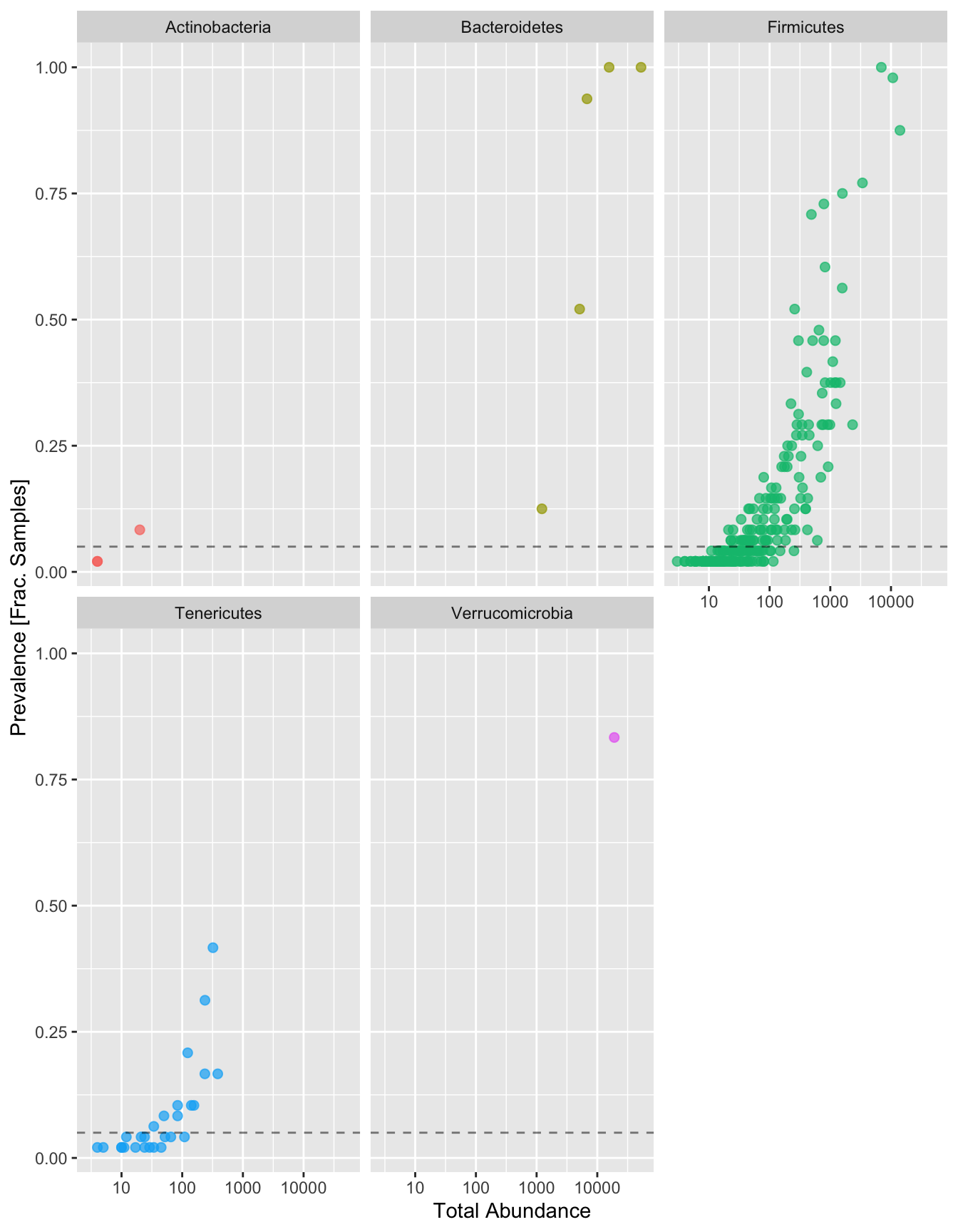
Now let’s physically remove those ASVs below that 5% prevalence threshold:
# Define prevalence threshold as 5% of total samples
prevalenceThreshold <- 0.05 * nsamples(ps)

# Execute prevalence filter, using `prune_taxa()` function
keepTaxa <- rownames(prevdf1)[(prevdf1$Prevalence >= prevalenceThreshold)]
ps1 <- prune_taxa(keepTaxa, ps)
And that’s it! You can now save your results to your computer using the following commands:
saveRDS(ps1, "ps1.rds")Visualization / Diversity
Phyloseq comes with a lot of great plot functions that are built around the ggplot2 package (ex. plot_ordination(), plot_bar()), but we’ll do it from “scratch” by extracting data frames from the phyloseq object and then plotting.
Phylum Relative Abundance
Before we can plot phylum relative abundance, we need to merge all ASV’s together that are within the same Phylum:
# Merge everything to the phylum level
ps1_phylum <- tax_glom(ps1, "Phylum", NArm = TRUE)
Then convert to relative abundance:
# Transform Taxa counts to relative abundance
ps1_phylum_relabun <- transform_sample_counts(ps1_phylum, function(OTU) OTU/sum(OTU) * 100)
Then extract the data from the phyloseq object:
taxa_abundance_table_phylum <- psmelt(ps1_phylum_relabun)And now we can plot a stacked bar plot:
StackedBarPlot_phylum <- taxa_abundance_table_phylum %>%
  ggplot(aes(x =Sample, y = Abundance, fill = Phylum)) +
  geom_bar(stat = "identity") +
  labs(x = "",
       y = "Relative Abundance",
       title = "Phylum Relative Abundance") +
  facet_grid(~ Diet, scales = "free") +
  theme(
    axis.text.x = element_text(size = 10, angle = 90, vjust = 0.5, hjust = 1),
    axis.text.y = element_text(size = 12),
    legend.text = element_text(size = 10),
    strip.text = element_text(size = 12)
  )

StackedBarPlot_phylum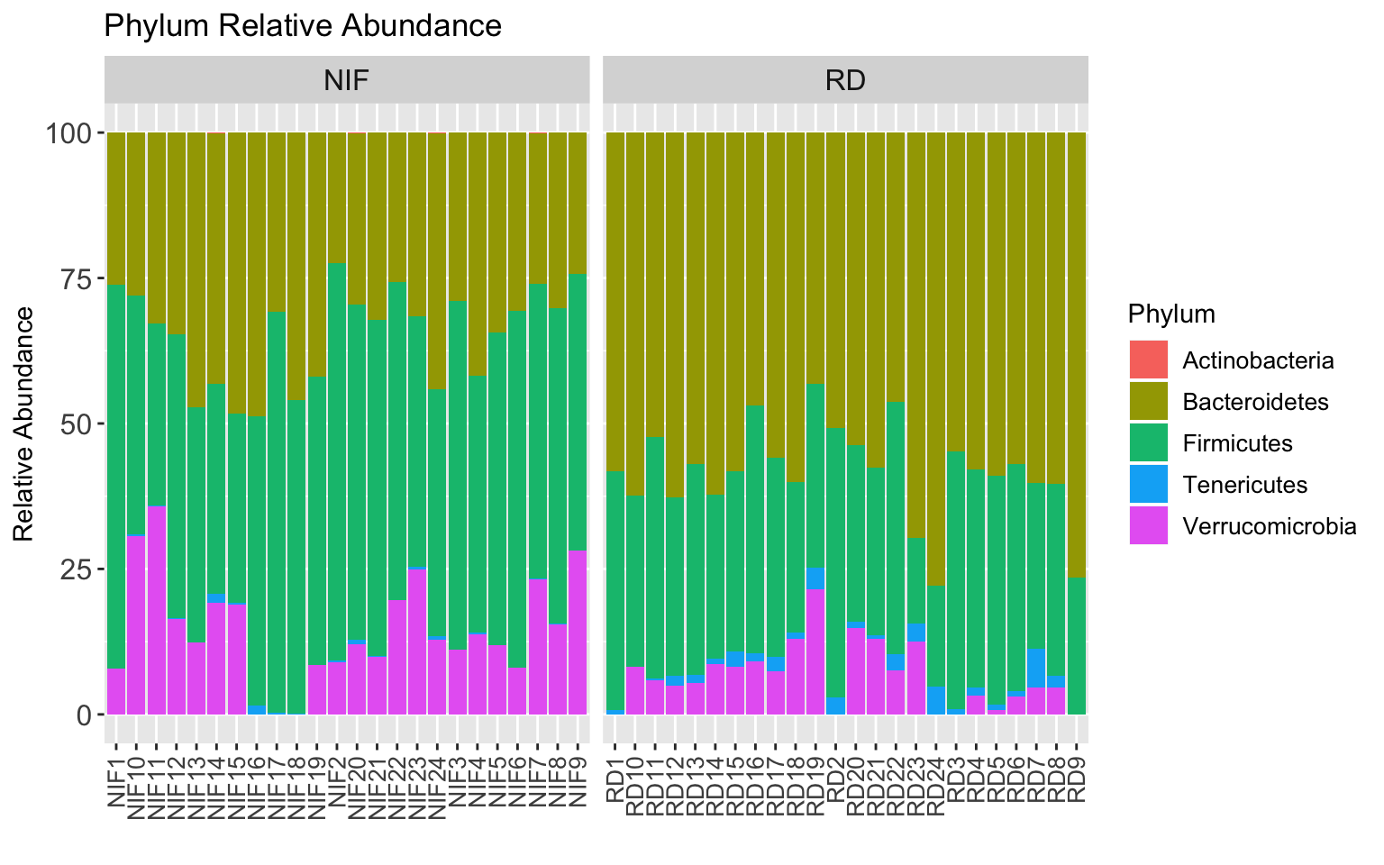
Looks like a difference for sure! Let’s plot each phylum as a box plot:
BoxPlot_phylum <- taxa_abundance_table_phylum %>%
  ggplot(aes(x =Phylum, y = Abundance, fill = Phylum)) +
  geom_boxplot() +
  labs(x = "",
       y = "Relative Abundance",
       title = "Phylum Relative Abundance") +
  facet_grid(~ Diet, scales = "free") +
  theme(
    axis.text.x = element_text(size = 10, angle = 90, vjust = 0.5, hjust = 1),
    axis.text.y = element_text(size = 12),
    legend.text = element_text(size = 10),
    strip.text = element_text(size = 12)
  )

BoxPlot_phylum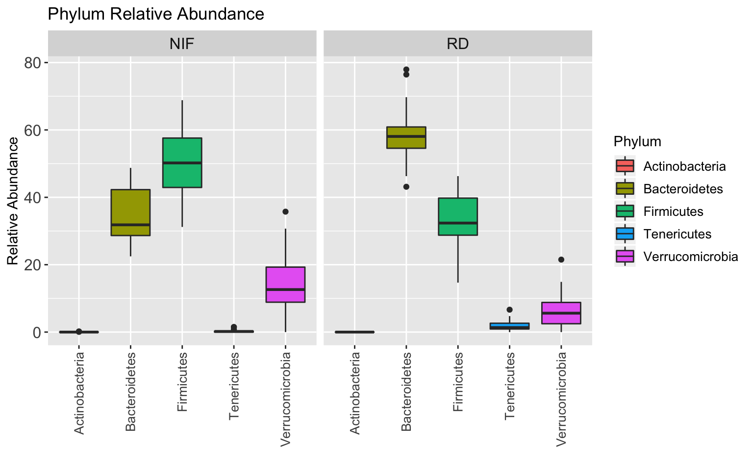
The ratio of Bacteroidetes to Firmicutes basically flips between the RD and NIF groups…cool!
Genus Relative Abundance
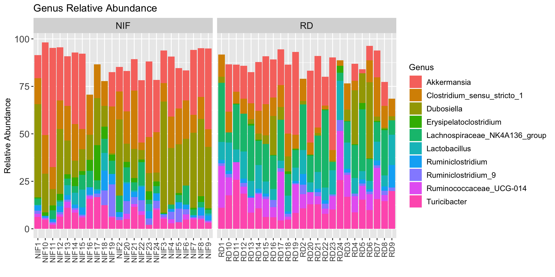
Let’s do the same thing as above but for the top 10 genera in our study:
ps1_genus <- tax_glom(ps1, "Genus", NArm = TRUE)

# Get top 10 genera
top10_genera <- names(sort(taxa_sums(ps1_genus), decreasing=TRUE))[1:10]

# Transform Taxa counts to relative abundance
ps1_genus_relabun <- transform_sample_counts(ps1_genus, function(OTU) OTU/sum(OTU) * 100)

# Extract the top 10 taxa and Regular Diet Samples
ps1_genus_top10 <- prune_taxa(top10_genera, ps1_genus_relabun)

# Convert into dataframe
taxa_abundance_table_genus <- psmelt(ps1_genus_top10)
Plot:
StackedBarPlot_genus <- taxa_abundance_table_genus %>%
  ggplot(aes(x =Sample, y = Abundance, fill = Genus)) +
  geom_bar(stat = "identity") +
  labs(x = "",
       y = "Relative Abundance",
       title = "Genus Relative Abundance") +
  facet_grid(~ Diet, scales = "free") +
  theme(
    axis.text.x = element_text(size = 10, angle = 90, vjust = 0.5, hjust = 1),
    axis.text.y = element_text(size = 12),
    legend.text = element_text(size = 10),
    strip.text = element_text(size = 12)
  )

StackedBarPlot_genus